时间复杂度

根据定义，时间复杂度指输入数据大小为 \(N\) 时，算法运行所需花费的时间。需要注意：

统计的是算法的「计算操作数量」，而不是「运行的绝对时间」。计算操作数量和运行绝对时间呈正相关关系，并不相等。算法运行时间受到「编程语言、计算机处理器速度、运行环境」等多种因素影响。例如，同样的算法使用 Python 或 C++ 实现、使用 CPU 或 GPU 、使用本地 IDE 或力扣平台提交，运行时间都不同。
体现的是计算操作随数据大小 \(N\) 变化时的变化情况。假设算法运行总共需要「 \(1\) 次操作」、「 \(100\) 次操作」，此两情况的时间复杂度都为常数级 \(O(1)\) ；需要「 \(N\) 次操作」、「 \(100N\) 次操作」的时间复杂度都为 \(O(N)\) 。

符号表示

根据输入数据的特点，时间复杂度具有「最差」、「平均」、「最佳」三种情况，分别使用 \(O\) , \(\Theta\) , \(\Omega\) 三种符号表示。以下借助一个查找算法的示例题目帮助理解。

题目： 输入长度为 \(N\) 的整数数组 nums ，判断此数组中是否有数字 \(7\) ，若有则返回 true ，否则返回 \(\text{false}\) 。

解题算法： 线性查找，即遍历整个数组，遇到 \(7\) 则返回 true 。

代码：

```Python [] def find_seven(nums): for num in nums: if num == 7: return True return False
1
2
3
4
5
6
7
8
```Java []
boolean findSeven(int[] nums) {
    for (int num : nums) {
        if (num == 7)
            return true;
    }
    return false;
}
C++ [] bool findSeven(vector<int>& nums) { for (int num : nums) { if (num == 7) return true; } return false; }

最佳情况 \(\Omega(1)\) ： nums = [7, a, b, c, ...] ，即当数组首个数字为 \(7\) 时，无论 nums 有多少元素，线性查找的循环次数都为 \(1\) 次；
最差情况 \(O(N)\) ： nums = [a, b, c, ...] 且 nums 中所有数字都不为 \(7\) ，此时线性查找会遍历整个数组，循环 \(N\) 次；
平均情况 \(\Theta\) ： 需要考虑输入数据的分布情况，计算所有数据情况下的平均时间复杂度；例如本题目，需要考虑数组长度、数组元素的取值范围等；

大 \(O\) 是最常使用的时间复杂度评价渐进符号，下文示例与本 LeetBook 题目解析皆使用 \(O\) 。

常见种类

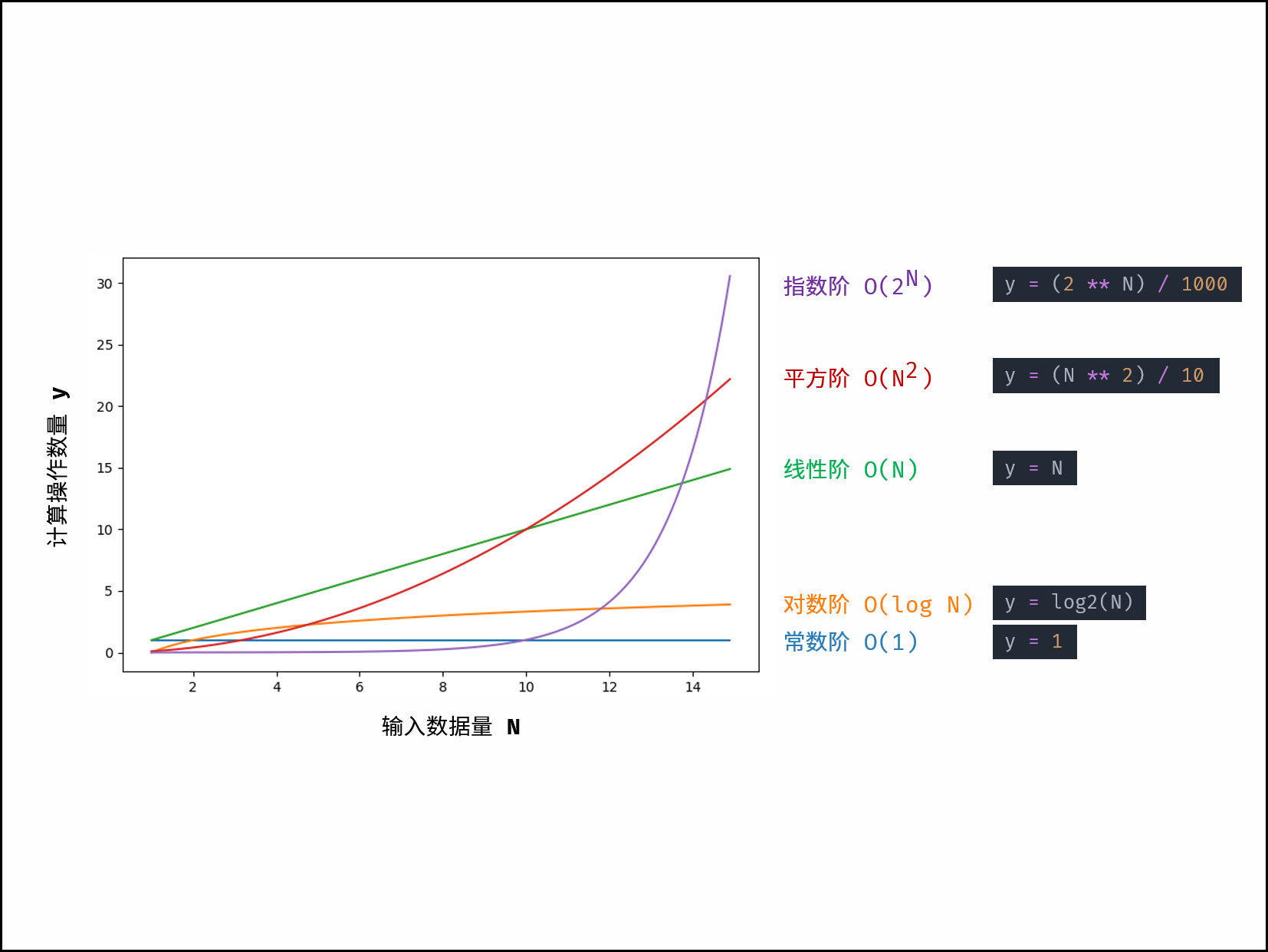
根据从小到大排列，常见的算法时间复杂度主要有：

\[ O(1) < O(\log N) < O(N) < O(N\log N) < O(N^2) < O(2^N) < O(N!) \]

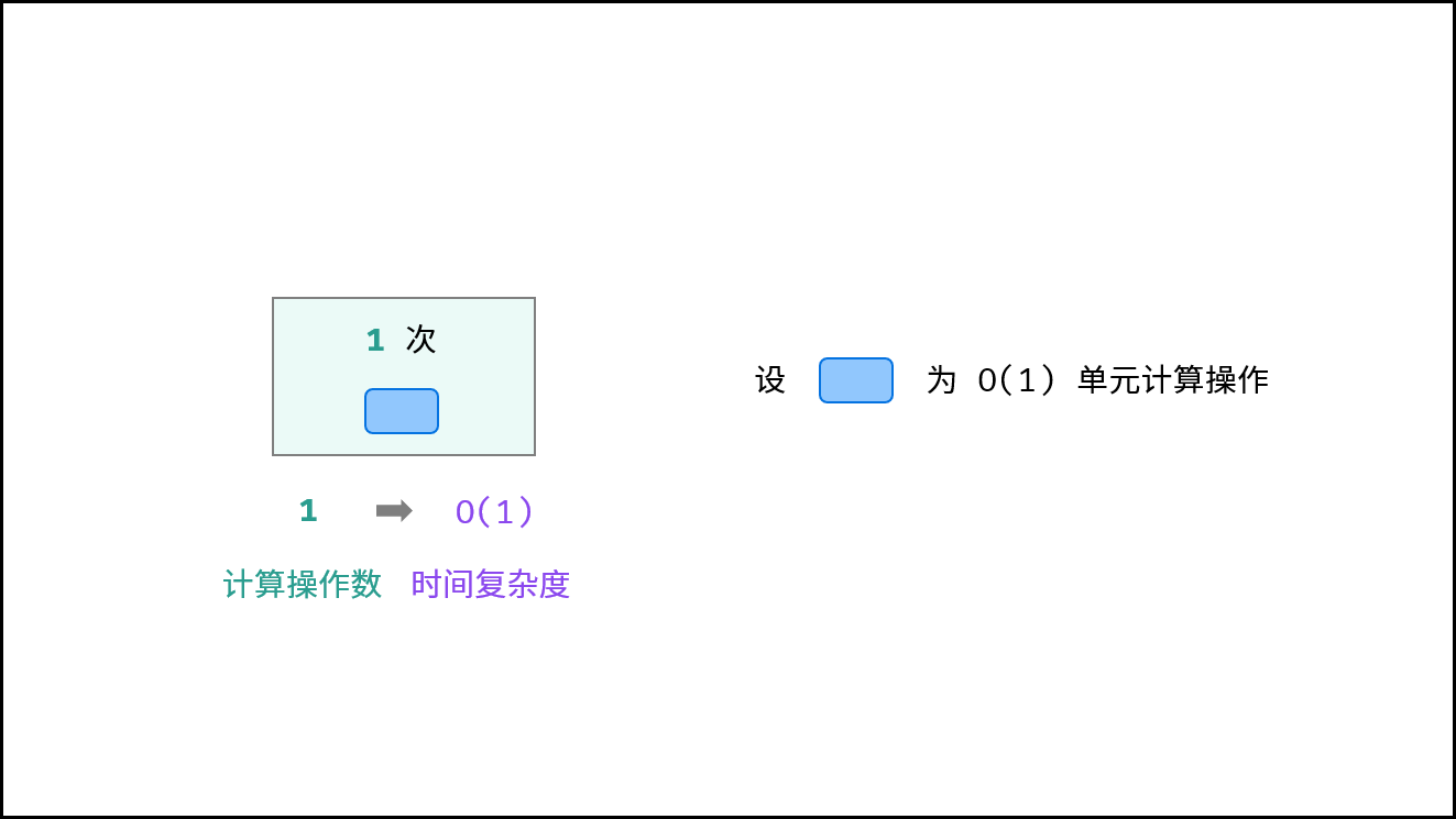
对于以下所有示例，设输入数据大小为 \(N\) ，计算操作数量为 \(count\) 。图中每个「蓝色方块」代表一个单元计算操作。

常数 \(O(1)\) ：

运行次数与 \(N\) 大小呈常数关系，即不随输入数据大小 \(N\) 的变化而变化。

```Python [] def algorithm(N): a = 1 b = 2 x = a * b + N return 1

```Java []
int algorithm(int N) {
    int a = 1;
    int b = 2;
    int x = a * b + N;
    return 1;
}

```C++ [] int algorithm(int N) { int a = 1; int b = 2; int x = a * b + N; return 1; }

对于以下代码，无论 $a$ 取多大，都与输入数据大小 $N$ 无关，因此时间复杂度仍为 $O(1)$ 。

```Python []
def algorithm(N):
    count = 0
    a = 10000
    for i in range(a):
        count += 1
    return count

```Java [] int algorithm(int N) { int count = 0; int a = 10000; for (int i = 0; i < a; i++) { count++; } return count; }

```C++ []
int algorithm(int N) {
    int count = 0;
    int a = 10000;
    for (int i = 0; i < a; i++) {
        count++;
    }
    return count;
}

{:width=500}

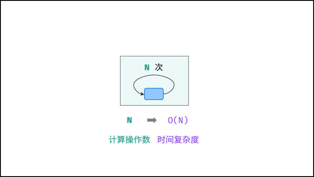
线性 \(O(N)\) ：

循环运行次数与 \(N\) 大小呈线性关系，时间复杂度为 \(O(N)\) 。

```Python [] def algorithm(N): count = 0 for i in range(N): count += 1 return count

```Java []
int algorithm(int N) {
    int count = 0;
    for (int i = 0; i < N; i++)
        count++;
    return count;
}

```C++ [] int algorithm(int N) { int count = 0; for (int i = 0; i < N; i++) count++; return count; }

对于以下代码，虽然是两层循环，但第二层与 $N$ 大小无关，因此整体仍与 $N$ 呈线性关系。

```Python []
def algorithm(N):
    count = 0
    a = 10000
    for i in range(N):
        for j in range(a):
            count += 1
    return count

```Java [] int algorithm(int N) { int count = 0; int a = 10000; for (int i = 0; i < N; i++) { for (int j = 0; j < a; j++) { count++; } } return count; }

```C++ []
int algorithm(int N) {
    int count = 0;
    int a = 10000;
    for (int i = 0; i < N; i++) {
        for (int j = 0; j < a; j++) {
            count++;
        }
    }
    return count;
}

{:width=500}

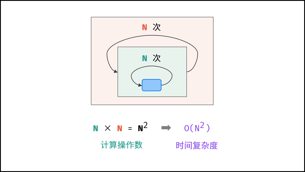
平方 \(O(N^2)\) ：

两层循环相互独立，都与 \(N\) 呈线性关系，因此总体与 \(N\) 呈平方关系，时间复杂度为 \(O(N^2)\) 。

```Python [] def algorithm(N): count = 0 for i in range(N): for j in range(N): count += 1 return count

```Java []
int algorithm(int N) {
    int count = 0;
    for (int i = 0; i < N; i++) {
        for (int j = 0; j < N; j++) {
            count++;
        }
    }
    return count;
}

```C++ [] int algorithm(int N) { int count = 0; for (int i = 0; i < N; i++) { for (int j = 0; j < N; j++) { count++; } } return count; }

以「冒泡排序」为例，其包含两层独立循环：

1. 第一层复杂度为 $O(N)$ ；
2. 第二层平均循环次数为 $\frac{N}{2}$ ，复杂度为 $O(N)$ ，推导过程如下：

$$
O(\frac{N}{2}) = O(\frac{1}{2})O(N) = O(1)O(N) = O(N)
$$

因此，冒泡排序的总体时间复杂度为 $O(N^2)$ ，代码如下所示。

```Python []
def bubble_sort(nums):
    N = len(nums)
    for i in range(N - 1):
        for j in range(N - 1 - i):
            if nums[j] > nums[j + 1]:
                nums[j], nums[j + 1] = nums[j + 1], nums[j]
    return nums

```Java [] int[] bubbleSort(int[] nums) { int N = nums.length; for (int i = 0; i < N - 1; i++) { for (int j = 0; j < N - 1 - i; j++) { if (nums[j] > nums[j + 1]) { int tmp = nums[j]; nums[j] = nums[j + 1]; nums[j + 1] = tmp; } } } return nums; }

```C++ []
vector<int> bubbleSort(vector<int>& nums) {
    int N = nums.size();
    for (int i = 0; i < N - 1; i++) {
        for (int j = 0; j < N - 1 - i; j++) {
            if (nums[j] > nums[j + 1]) {
                swap(nums[j], nums[j + 1]);
            }
        }
    }
    return nums;
}

{:width=450}

指数 \(O(2^N)\) ：

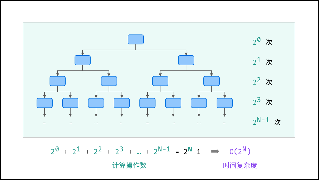
生物学科中的 “细胞分裂” 即是指数级增长。初始状态为 \(1\) 个细胞，分裂一轮后为 \(2\) 个，分裂两轮后为 \(4\) 个，……，分裂 \(N\) 轮后有 \(2^N\) 个细胞。

算法中，指数阶常出现于递归，算法原理图与代码如下所示。

```Python [] def algorithm(N): if N <= 0: return 1 count_1 = algorithm(N - 1) count_2 = algorithm(N - 1) return count_1 + count_2

```Java []
int algorithm(int N) {
    if (N <= 0) return 1;
    int count_1 = algorithm(N - 1);
    int count_2 = algorithm(N - 1);
    return count_1 + count_2;
}

```C++ [] int algorithm(int N) { if (N <= 0) return 1; int count_1 = algorithm(N - 1); int count_2 = algorithm(N - 1); return count_1 + count_2; }

![Picture5.png](https://pic.leetcode-cn.com/1623519242-XLBkIT-Picture5.png){:width=600}

### 阶乘 $O(N!)$ ：

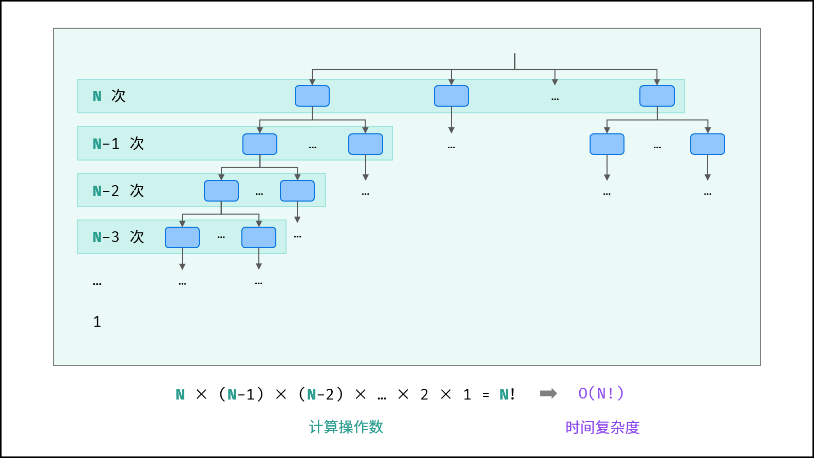
阶乘阶对应数学上常见的 “全排列” 。即给定 $N$ 个互不重复的元素，求其所有可能的排列方案，则方案数量为：

$$
N \times (N - 1) \times (N - 2) \times \cdots \times 2 \times 1 = N!
$$

如下图与代码所示，阶乘常使用递归实现，算法原理：第一层分裂出 $N$ 个，第二层分裂出 $N - 1$ 个，…… ，直至到第 $N$ 层时终止并回溯。

```Python []
def algorithm(N):
    if N <= 0: return 1
    count = 0
    for _ in range(N):
        count += algorithm(N - 1)
    return count

```Java [] int algorithm(int N) { if (N <= 0) return 1; int count = 0; for (int i = 0; i < N; i++) { count += algorithm(N - 1); } return count; }

```C++ []
int algorithm(int N) {
    if (N <= 0) return 1;
    int count = 0;
    for (int i = 0; i < N; i++) {
        count += algorithm(N - 1);
    }
    return count;
}

{:width=600}

对数 \(O(\log N)\) ：

对数阶与指数阶相反，指数阶为 “每轮分裂出两倍的情况” ，而对数阶是 “每轮排除一半的情况” 。对数阶常出现于「二分法」、「分治」等算法中，体现着 “一分为二” 或 “一分为多” 的算法思想。

设循环次数为 \(m\) ，则输入数据大小 \(N\) 与 \(2 ^ m\) 呈线性关系，两边同时取 \(log_2\) 对数，则得到循环次数 \(m\) 与 \(\log_2 N\) 呈线性关系，即时间复杂度为 \(O(\log N)\) 。

```Python [] def algorithm(N): count = 0 i = N while i > 1: i = i / 2 count += 1 return count

```Java []
int algorithm(int N) {
    int count = 0;
    float i = N;
    while (i > 1) {
        i = i / 2;
        count++;
    }
    return count;
}

```C++ [] int algorithm(int N) { int count = 0; float i = N; while (i > 1) { i = i / 2; count++; } return count; }

如以下代码所示，对于不同 $a$ 的取值，循环次数 $m$ 与 $\log_a N$ 呈线性关系 ，时间复杂度为 $O(\log_a N)$ 。而无论底数 $a$ 取值，时间复杂度都可记作 $O(\log N)$ ，根据对数换底公式的推导如下：

$$
O(\log_a N) = \frac{O(\log_2 N)}{O(\log_2 a)} = O(\log N)
$$

```Python []
def algorithm(N):
    count = 0
    i = N
    a = 3
    while i > 1:
        i = i / a
        count += 1
    return count

```Java [] int algorithm(int N) { int count = 0; float i = N; int a = 3; while (i > 1) { i = i / a; count++; } return count; }

```C++ []
int algorithm(int N) {
    int count = 0;
    float i = N;
    int a = 3;
    while (i > 1) {
        i = i / a;
        count++;
    }
    return count;
}

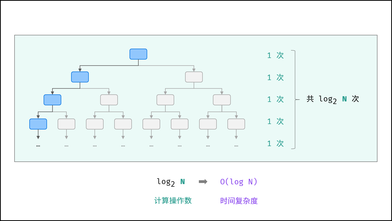
如下图所示，为二分查找的时间复杂度示意图，每次二分将搜索区间缩小一半。

{:width=600}

线性对数 \(O(N \log N)\) ：

两层循环相互独立，第一层和第二层时间复杂度分别为 \(O(\log N)\) 和 \(O(N)\) ，则总体时间复杂度为 \(O(N \log N)\) ；

```Python [] def algorithm(N): count = 0 i = N while i > 1: i = i / 2 for j in range(N): count += 1

```Java []
int algorithm(int N) {
    int count = 0;
    float i = N;
    while (i > 1) {
        i = i / 2;
        for (int j = 0; j < N; j++)
            count++;
    }
    return count;
}

C++ [] int algorithm(int N) { int count = 0; float i = N; while (i > 1) { i = i / 2; for (int j = 0; j < N; j++) count++; } return count; }

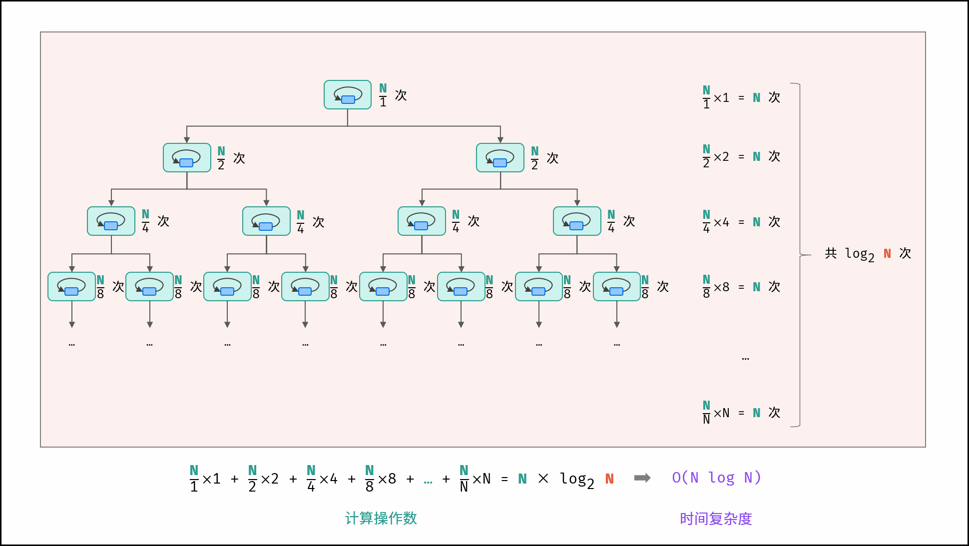
线性对数阶常出现于排序算法，例如「快速排序」、「归并排序」、「堆排序」等，其时间复杂度原理如下图所示。

示例题目

以下列举本 LeetBook 中各时间复杂度的对应示例题解，以帮助加深理解。

时间复杂度	示例题解
\(O(1)\)	砍竹子 I、文物朝代判断
\(O(\log N)\)	Pow(x, n)、统计目标成绩的出现次数
\(O(N)\)	训练计划 III、斐波那契数
\(O(N \log N)\)	破解闯关密码、交易逆序对的总数
\(O(N^2)\)	验证二叉搜索树的后序遍历序列、招式拆解 I
\(O(N!)\)	套餐内商品的排列顺序